GPR survey processing using OpendTect

A GPR survey was performed with a GPS running to collect position of irregular path along the various transects. The objective is to display all GPR traces in a consistent geographic setting and framework. The start and end GPS (WGS84/UTM33N) coordinates were manually picked and the ASCII array holding the GPR voltage as a function of time (B-scans) is prefixed with the interpolated position. This is the dataset to be included in OpendTect.

1. "I will set up a survey myself" -> Create new survey -> Enter by hand (Time)
   
   
   
2. Survey ranges: In-line range from 0 to 1 with step 1, Crossline range from 0 to 1 with step 1, Z range from 0 to 4095 with 1 ms steps (milliseconds).
   
   
   
3. The objective of mapping in-line/cross-line coordinates with geographic coordinates is met by filling the relations between 3 points defining a plane in each coordinate framework. Here we selected a single in-line and cross-line range so that the geographical coordinates of the field, here from (438790,8759135) bottom left corner to (439230,8759556) top right corner (WGS84/UTM33N) must span the (0,0) to (1,1) range as defined in the following (left) and we check after hitting Apply that the linear transform matches expectations, most easily with the bottom left corner at origin:
   
   
4. The survey definition is now complete, we are ready to import 2D GPR B-scan datasets in the 3D scene of OpendTect:
   
   
5. ASCII files with 4095 samples/trace and quite a few traces for each GPR scan is prefixed by the interpolated location between the starting and ending point using a few lines of GNU/Octave code

   load position.33N  % 2 columns with X and Y of start and end of each trace
   
   dl=dir('*-main');  % load GPR trace, ASCII file
   for dn=1:length(dl)
   	x=load(dl(dn).name);
   	X=linspace(position(2*dn-1,1),position(2*dn-0,1),size(x)(1));
   	Y=linspace(position(2*dn-1,2),position(2*dn-0,2),size(x)(1));
   	x=[(X') (Y') x];
   	nom=[dl(dn).name,".pos33N"]
   	eval(["save -text ",nom," x"])
   end
   	

   
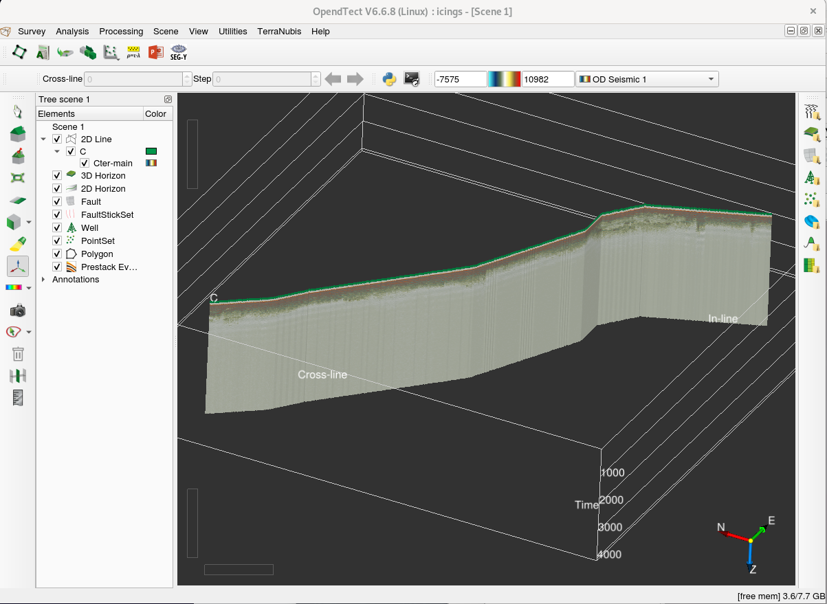
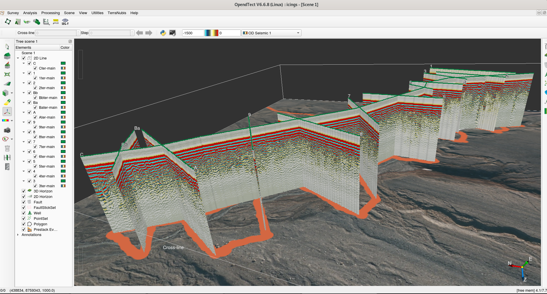
   resulting files looking like
   

   439154 8759300 -759 -751 -748 -744 -746 -751 -755 ...
   439153 8759299 -771 -750 -755 -756 -747 -758 -758 ...
   439153 8759299 -766 -754 -749 -755 -751 -748 -760 ...
   439153 8759299 -765 -747 -751 -746 -752 -748 -748 ...
   439153 8759299 -758 -753 -756 -742 -749 -751 -756 ...
   439153 8759299 -768 -763 -755 -757 -749 -749 -756 ...
   439153 8759299 -772 -764 -744 -750 -750 -757 -753 ...
   439153 8759299 -769 -767 -752 -750 -754 -748 -748 ...
   ...
   	

   with 4097=4095+2 items on each line and number of traces lines, no leading white space following save -text from Octave and removal of the header and the leading space
6. Survey -> Import -> Seismic Data -> Simple File -> Line ... File Type ASCII, Input File selected and making sure the file is properly read (Examine) and checking all entries, most significantly the number of samples/line
   
   
7. Having made sure Examine displays fine, Traces Start with a position = Yes ; Trace number included = No ; Trace number definition: start at 1, step 1 ; File start contains sampling info = No ; Sampling info: start=0 ; step = 1 ms ; #samples=4095 ; Output 2D Data same as filename and Line name set
   
   
8. Once the GPR B-scan dataset has been loaded, back to the main window and 2D Line -> Add
   
9. Make sure the trace is visible in the surveyed area and that the track matches the expected location as was observed initially in QGis. If all fits, then Select Attribute -> Stored 2D Data will display the GPR B-scan
   
10. Scale the Z-axis using View -> ZScale and possibly change the color range of each B-scan using 2D Line -> Edit Color Settings to enhance contrast

11. Repeat for all traces since I could not find how to automate the process
12. 
13. We might wish to add a background map for documenting the geographical context. Back to QGis where the GPS traces are overlaid on the aerial image, Export Map to Image ... and selecting the exact same range as was documented in OpendTect Survey settings
    
14. Using the Scene settings, add the map as a Bottom image
    
15. Finally, the depth range might be too large and selecting the Z-location of the backgroun map helps focus on the relevant features of the GPR scans, here in the shallowest areas